Computing Duck

It’s been a long time since I last used MATLAB so I was quite excited when I had a chance to do so recently. Expanding upon the general idea, I decided to rewrite the function to automate a few things and to allow a few more options regarding the type of motion being examined. Hopefully this winds up being a bit more demonstrative and will give me the opportunity to finally write a tutorial-style article regarding these operations.

Note that I do not presume anything near expertise, I have merely written something which works and I feel that its explanation is a worthy exercise and may serve as a useful demonstration for those who’ve not been introduced to or those who have not grasped the concept of instantaneous velocity.

If you only wish to see the finished result then click here

So, to reiterate, the purpose of this code is to help demonstrate the effect of temporal interval on both the value and the accuracy of measures of the velocity of some object undergoing motion within one dimension. Thus, we must start with at least two vectors of data (time and position) which we shall neatly encapsulate within a structure which I call physbb as this was originally a response to a query on a physics message board.

Time:

physqbb.t=t1:((t2-t1)/obs):t2; % Generate t ranging from t1 to t2 with
%obs number of equally spaced observations.

This is straightforward. Times t1 and t2 are your upper and lower bounds of observation and you have obs number of data points being recorded.

Position:

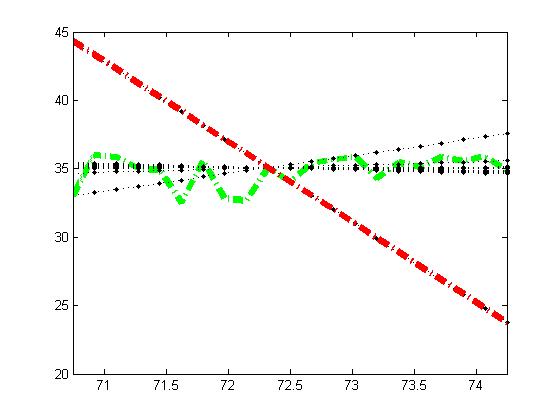
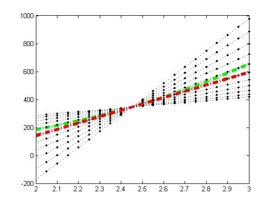
if fit=='normal'
    physqbb.d=normrnd(A,B,1,obs+1); % Generate random numbers for each value of t
    %based on a normal distribution with mu=35, sigma=10.
end
if fit=='polyva'
    physqbb.d=(D.*physqbb.t.^3)+(C.*physqbb.t.^2)+(B.*physqbb.t)+A;
end
if fit=='fourie'
    physqbb.d=(C.*sin(physqbb.t))+(B.*cos(physqbb.t))+A;
end

These options for generating the position data make up the largest part of the difference between this and the original iteration of this code. If ‘normal’, ‘polyva’ or ‘fourie’ are specified as the function type then the position data will respectively b:: generated from a normal distribution with mu=A, and sigma=B, calculated from a polynomial equation (maximum order is 3rd but that can easily be changed) polynomial coefficients A, B, C and D, or calculated from a fourier equation with sin and cosine amplitudes C and B and A displacement.

Now that we’ve generated the relevant data, our next step is to fit lines passing through the position midway between t1 and t2 and the position at a number of equally spaced points of observations. These lines constitute measures of average velocity within the specified time frame.

Velocity-line generation:

j=-49:5:51;
physqbb.dt(1:21)=physqbb.t(ceil(obs/2)+j(1:21))-physqbb.t(ceil(obs/2));
physqbb.dx(1:21)=physqbb.d(ceil(obs/2)+j(1:21))-physqbb.d(ceil(obs/2));
for i=1:21
physqbb.v(i)=physqbb.dx(i)/physqbb.dt(i);
physqbb.b(i)=physqbb.d(ceil(obs/2))-(physqbb.v(i).*physqbb.t(ceil(obs/2)));
physqbb.l(i,:)=(physqbb.v(i).*physqbb.t)+physqbb.b(i);
end

As velocity is a measure of , physbb.v is derived from the division of physbb.dx by physbb.dt – simple enough.

physqbb.b is the position axis intercept for the line with some slope physqbb.v passing through some point [physqbb.d(ceil(obs/2)),physqbb.t(ceil(obs/2))] – which is to say the position at the midway point between t1 and t2.

physqbb.l is an array of position by time data which were generated based on the linear equation.

j and i are a bit like relics of the original code as I chose only to capture a discrete amount of fits spaced 5 intervals of physqbb.t apart. These can certainly be rewritten for more flexibility w/regard to the interval spacing but I wonder as to the usefulness of doing so.

The final step is to plot these lines:
Plotting

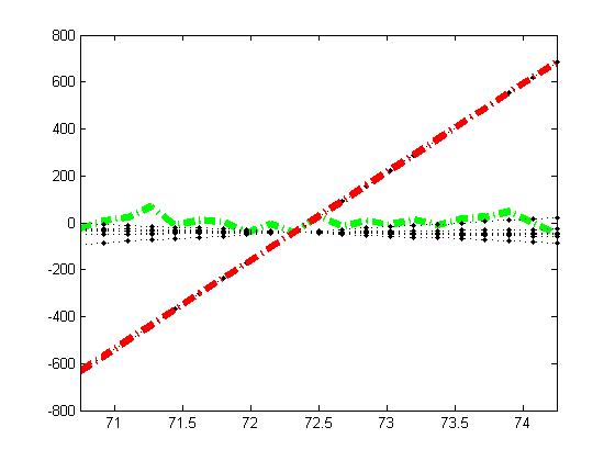
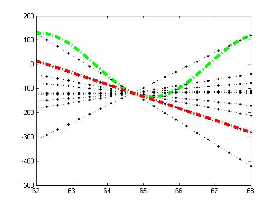
plot(physqbb.t,physqbb.d,'-.g','LineWidth',5);
hold
for i=1:2:21
plot(physqbb.t,physqbb.l(i,:),':.k');
end
plot(physqbb.t,physqbb.l(11,:),'-.r','LineWidth',5);
hold off
set(gca, 'xlim', [(mean([t1 t2])-10*((t2-t1)/obs)) (mean([t1 t2])+10*((t2-t1)/obs))],'ylimMode', 'auto')

Nothing special here, just plotting the lines and then making the original data and fit derived from the smallest interval stand out.

Some examples:
Normal

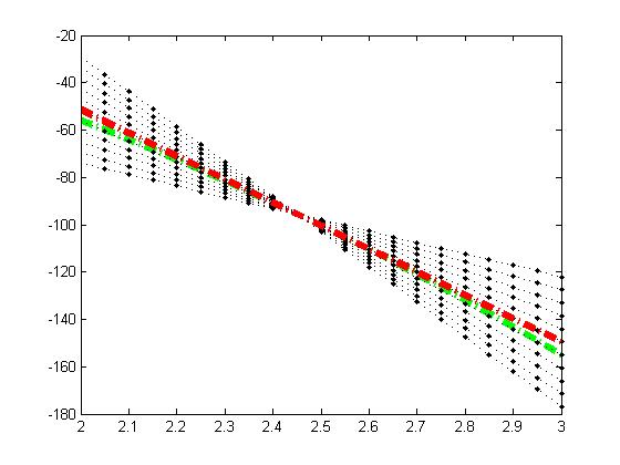
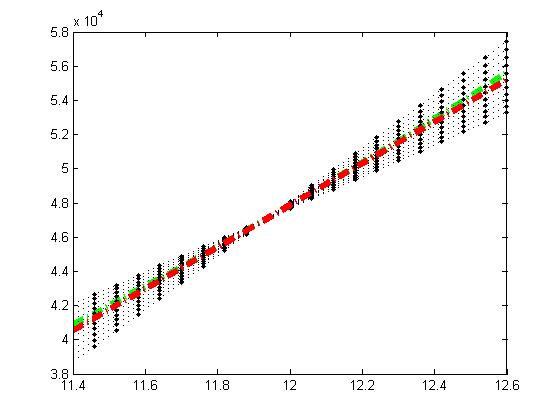
Polynomial

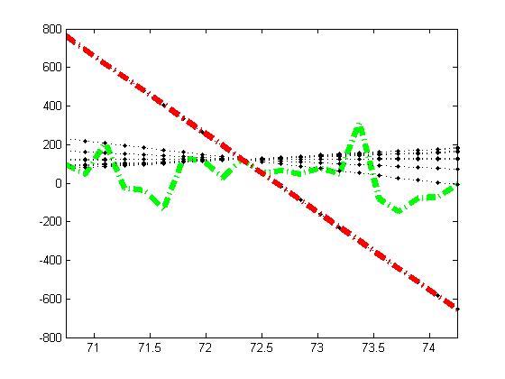
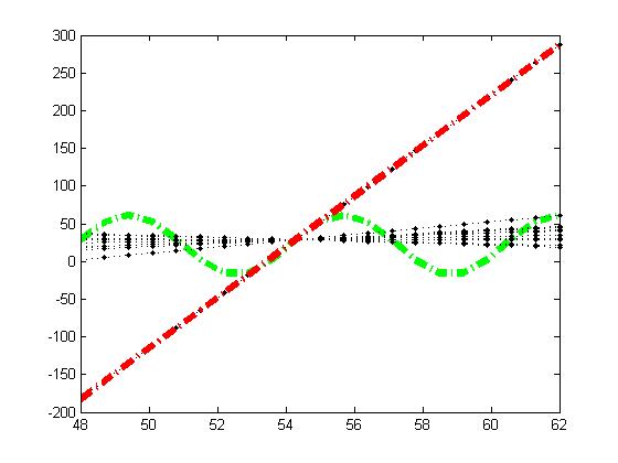
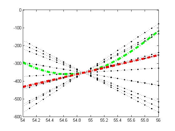
Fourier

Exercises:
For anyone who has found any parts of this explanation beneficial, a few exercises based on this theme may prove worthwhile:
1. It is the nature of time to increment only in the forwards direction. Write either a warning or error code for the case when t1>t2.
2. Add options to create a few different distributions/equations/any other sort of algorithm for the generation of the raw position data.
3. Notice the abbreviation for the generation type in this code. This is due to the use of == which necessitates equal dimensions of string length. Use MATLAB’s suggested alternative code to allow strings of varying lengths.
4. Compare the goodness of fit of all the lines for segments of varying intervals after the initial time of observation.
5. Find the acceleration during the periods of observation.
6. Use the relative change in position to create a functionally determined bounding scheme for Xlim and Ylim.